

Teaching Linear Programming using Microsoft Excel Solver
Ziggy MacDonald
University of Leicester
Linear programming (LP) is one of the most widely applied O.R. techniques and owes its popularity principally to George Danzig's simplex method (Danzig 1963) and the revolution in computing. It is a very powerful technique for solving allocation problems and has become a standard tool for many businesses and organisations. Although Danzig's simplex method allows solutions to be generated by hand, the iterative nature of producing solutions is so tedious that had the computer never been invented then linear programming would have remained an interesting academic idea, relegated to the mathematics classroom. Fortunately, computers were invented and as they have become so powerful for so little cost, linear programming has become possibly one of the most widespread uses for a personal PC.
There are of course numerous software packages which are dedicated to solving linear programs (and other types of mathematical program), of which possibly LINDO, GAMS and XPRESS-MP are the most popular. All these packages tend to be DOS based and are intended for a specialist market which requires tools dedicated to solving LPs. In recent years, however, several standard business packages, such as spreadsheets, have started to include an LP solving option, and Microsoft Excel is no exception. The inclusion of an LP solving capability into applications such as Excel is attractive for at least two reasons. Firstly, Excel is perhaps the most popular spreadsheet used both in business and in universities and as such is very accessible. Second to this, the spreadsheet offers very convenient data entry and editing features which allows the student to gain a greater understanding of how to construct linear programs.
To use Excel to solve LP problems the Solver add-in must be included. Typically this feature is not installed by default when Excel is first setup on your hard disk. To add this facility to your Tools menu you need to carry out the following steps (once-only):
- Select the menu option Tools | Add_Ins (this will take a few moments to load the necessary file).
- From the dialogue box presented check the box for Solver Add-In.
- On clicking OK, you will then be able to access the Solver option from the new menu option Tools | Solver (which appears below Tools | Scenarios ...)
To illustrate Excel Solver I will consider Hillier & Lieberman's reasonably well known example, the Wyndor Glass Co. problem (Hillier & Lieberman, 1995). The problem concerns a glass manufacturer which uses three production plants to assemble its products, mainly glass doors (x1) and wooden frame windows (x2). Each product requires different times in the three plants and there are certain restrictions on available production time at each plant. With this information and a knowledge of contributions to profit of the two products the management of the company wish to determine what quantities of each product they should be producing in order to maximise profits. In other words, the Wyndor Glass Co. problem is a classic, albeit very simple, product-mix problem.
The problem is formulated as the following linear program:
     max z = 3x1 + 2x2   (objective)

     subject to       x1 <= 4  (Plant One)
                     2x2 <= 12 (Plant Two)
               3x1 + 2x2 <= 18 (Plant Three)

                  x1, x2 >=  0  (Non-negativity requirements)

     where          z = total profit per week
               x1 = number of batches of doors produced per week
               x2 = number of batches of windows produced per week.
Having formulated the problem, and yours may have substantially more decision variables and constraints, you can then proceed to entering it into Excel. The best approach to entering the problem into Excel is first to list in a column the names of the objective function, decision variables and constraints. You can then enter some arbitrary starting values in the cells for the decision variables, usually zero, shown in Figure One. Excel will vary the values of the cells as it determines the optimal solutions. Having assigned the decision variables with some arbitrary starting values you can then use these cell references explicitly in writing the formulae for the objective function and constraints, remembering to start each formula with an '=' .
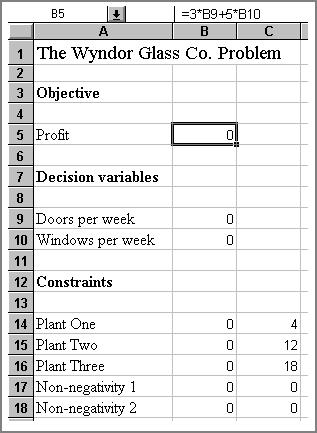
Figure One: Setting up the problem in Excel
Entering the formulae for the objective and constraints, the objective function in B5 will be given by :
=3*B9+2*B10
The constraints will be given by (putting the right hand side {RHS} values in the adjacent cells):
Plant One (B14)     =B9
Plant Two (B15)     =2*B10
Plant Three    (B16)     =3*B9+2*B10
Non-neg 1      (B17)     =B9
Non neg 2      (B19)     =B10
You are now ready to use Solver.
On selecting the menu option Tools | Solver the dialogue box shown in Figure Two is revealed, and if you select the objective cell before invoking Solver the correct Target Cell will be identified. This is the value Solver will attempt either to maximise or minimise.
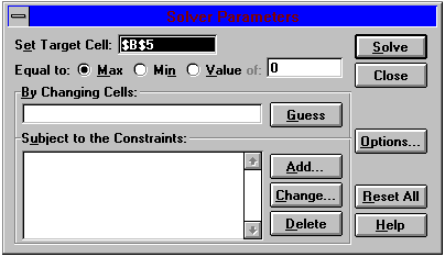
Figure Two: The Solver Dialogue Box
Select whether you wish to minimise this or maximise the problem, in this case you would want to set the target cell (the objective) to a Max. Note that you can use Solver to find the outcome that will achieve a specified value for the target cell by clicking 'Value of:'. In doing this you can use Solver as a glorified goal seeker.Next you enter the range of cells you want Solver to vary, the decision variables. Click on the white box and select cells B9 & B10, or alternatively type them in. Note that you can try to get Solver to guess which cells you want to vary by clicking the 'Guess' button. If you have defined your problem in a logical way Solver should usually get these right.
You can now enter the constraints by first clicking the 'Add ..' button. This reveals the dialogue box shown in Figure Three.
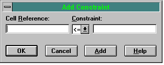
Figure Three: Entering Constraints
The cell reference is to the cell containing your constraint formula, so for the Plant One constraint you enter B14. By default <= is selected but you can change this by clicking on the drop down arrow to reveal a list of other constraint types. In the right hand white box you enter the cell reference to the cell containing the RHS value, which for the Plant One constraint is cell C14. You then click 'Add' to add the rest of the constraints, remembering to include the non-negativity constraints.
Having added all the constraints, click 'OK' and the Solver dialogue box should look like that shown in Figure Four.
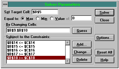
Figure Four: The Completed Solver Dialogue Box
Before clicking 'Solve' it is good practice when doing LPs to go into the Options and check the 'Assume Linear Model' box, unless, of course, your model isn't linear (Solver can handle most mathematical program types, including non-linear and integer problems). Doing this can speed up the length of time taken for Solver to find a solution to the problem and in fact, it will also ensure the correct result and quite importantly, provide the relevant sensitivity report. Having selected this option you are now ready to Click 'Solve' and see Solver find the optimal values for doors and windows. On doing this, at the bottom of the screen Excel will inform you of Solver's progress, then on finding an optimal solution the dialogue box shown in Figure Five will appear. You will also observe that Solver has altered all the values in your spreadsheet, replacing them with the optimal results.
You can use the Solver Results dialogue box to generate three reports. To select all three at once, either hold down CTRL and click each one in turn or drag the mouse over all three.
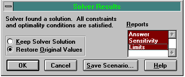
Figure Five: Solver Results
At the same time it's often a good idea to get Solver to restore your original values in the spreadsheet so that you can return to the original problem formulation and make adjustments to the model such as altering the availability of resources. The three reports are generated in new sheets in the current workbook of Excel.
The Answer Report gives details of the solutions (in this case, profit is maximised at 36 when 2 doors per week are produced and 6 windows per week - not a particularly busy firm!) and information concerning the status of each constraint with accompanying slack/surplus values is provided. The Sensitivity Report for the Wyndor problem, which provides information about how sensitive your solution is to changes in the constraints, is shown in Figure Six.
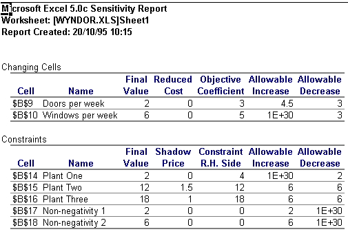
Figure Six: Sensitivity Report for Wyndor
As you can see from Figure Six, the report is fairly standard, providing information on shadow values, reduced cost and the upper and lower limits for the decision variables and constraints. The Limits Report also provides sensitivity information on the RHS values. All the reports can simply be copied and pasted into Word and this is perhaps one of the big advantages of using Excel over a DOS based LP solver. Although the reports paste into Word as tables, they are easily converted into text and can then be manipulated if one is producing a written report on your finding.
Finally, there are several options to Solver that can allow you to amend/intervene in the solution generating process. The 'Options' button in the Solver dialogue box reveals the dialogue box shown in Figure Seven. You can use this to affect how accurate your solution is, how much 'effort' Solver puts into to finding the solution and whether you want to see the results of each iteration.
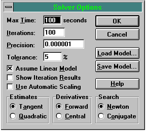
Figure Seven: Solver Options
The Tolerance option is only required for integer programs (IP), and allows Solver to use 'near integer' values, within the tolerance you specify, and this helps speed up the IP calculations. Checking the Show Iteration Results box allows you to see each step of the calculation, but be warned, if your model is complex this can take an inordinate length of time. Use Automatic Scaling is useful if there is a huge difference in magnitude between your decision variables and the objective value.
The bottom three options, Estimates, Derivatives and Search affect the way Solver approaches finding a basic feasible solution, how Solver finds partial differentials of the objective and constraints, and how Solver decides which way to search for the next iteration. Essentially the options affect how solver uses memory and the number of calculations it makes. For most LP problems, they are best left as the default values.
The 'Save Model' button is very useful, particularly if you save your model as a named scenario. Clicking this button allows you to assign a name to the current values of your variable cells. This option then allows you to perform further 'what-if' analysis on a variety of possible alternative outcomes - very useful for exploring your model in greater detail.
In conclusion, Excel Solver provides a simple, yet effective, medium for allowing users to explore linear programs. It can be used for large problems containing hundreds of variables and constraints, and does these relatively quickly, but as a teaching tool using small illustrative problems it is very potent, particularly as the student must appreciate the structure of a LP when entering it into the spreadsheet.
On the downside, you can't view the Tableau as it is generated at each iteration and so those teachers who would want their students to be proficient in the manual methods of LP would find Solver less superior to, say, Lindo, which does allow this. It does, however, produce a superior set of results and sensitivity reports when compared to Lindo, and, due to the spreadsheet nature, does allow the student very quickly to observe the effects of any changes made to constraints or the objective function.
This is particularly noticeable as the model formulation is easily accessible at the same time as the model results, these being simply placed in adjacent worksheets, accessible with a simple mouse click. Overall, using Excel, which is familiar to a large number of students, provides a rich environment for teaching linear programming and it allows students to explore their models in a structured, yet flexible, way.
References
- George B. Dantzig (1963) "Linear Programming and Extensions", Princeton University Press, Princeton, N.J.
- Frederick Hillier & Gerald Lieberman (1995) "Introduction to Operations Research", sixth edition, McGraw-Hill
- The Cobb Group (1994) "Running Excel 5 for Windows", fourth edition, Microsoft Press
The author may be contacted at the following address:
Ziggy MacDonald, Department of Economics, University of Leicester, University Road, Leicester LE1 7RH, United Kingdom. Telephone +44 (0)116 252 2894, Fax +44 (0) 252 2908, e-mail abm1@le.ac.uk


0 comments:
Post a Comment